Chapter 3 Structural equation modeling
3.0.1 The classic example of a structural equation model
3.0.2 Fitting a full structural equation model
library(haven)

sem.data <- read_dta("http://www.stata-press.com/data/r13/sem_sm2.dta")
sem.data <- as.matrix(sem.data)

library(lavaan)
sem.model <- '
  # latent variable measurements
  alien67 =~ anomia67 + pwless67
  alien71 =~ anomia71 + pwless71
  ses66 =~ educ66 + occstat66

  # structural models
  alien67 ~ ses66
  alien71 ~ alien67 + ses66
'

sem.fit <- sem(sem.model, sample.cov = sem.data, sample.nobs = 933)
summary(sem.fit, standardized = TRUE)
## lavaan 0.6-9 ended normally after 26 iterations
##
## Estimator ML
## Optimization method NLMINB
## Number of model parameters 15
##
## Number of observations 933
##
## Model Test User Model:
##
## Test statistic 71.697
## Degrees of freedom 6
## P-value (Chi-square) 0.000
##
## Parameter Estimates:
##
## Standard errors Standard
## Information Expected
## Information saturated (h1) model Structured
##
## Latent Variables:
## Estimate Std.Err z-value P(>|z|) Std.lv Std.all
## alien67 =~
## anomia67 1.000 0.812 0.813
## pwless67 0.999 0.047 21.436 0.000 0.811 0.812
## alien71 =~
## anomia71 1.000 0.839 0.840
## pwless71 0.951 0.045 21.265 0.000 0.798 0.798
## ses66 =~
## educ66 1.000 0.832 0.833
## occstat66 0.779 0.063 12.417 0.000 0.648 0.649
##
## Regressions:
## Estimate Std.Err z-value P(>|z|) Std.lv Std.all
## alien67 ~
## ses66 -0.553 0.051 -10.888 0.000 -0.567 -0.567
## alien71 ~
## alien67 0.685 0.052 13.177 0.000 0.663 0.663
## ses66 -0.153 0.047 -3.237 0.001 -0.151 -0.151
##
## Variances:
## Estimate Std.Err z-value P(>|z|) Std.lv Std.all
## .anomia67 0.339 0.029 11.712 0.000 0.339 0.339
## .pwless67 0.340 0.029 11.769 0.000 0.340 0.341
## .anomia71 0.295 0.030 9.919 0.000 0.295 0.295
## .pwless71 0.363 0.029 12.428 0.000 0.363 0.363
## .educ66 0.306 0.052 5.906 0.000 0.306 0.307
## .occstat66 0.579 0.040 14.319 0.000 0.579 0.579
## .alien67 0.448 0.040 11.242 0.000 0.679 0.679
## .alien71 0.298 0.031 9.664 0.000 0.424 0.424
## ses66 0.693 0.067 10.410 0.000 1.000 1.000library(semPlot)
semPaths(object = sem.fit, what = "std", edge.label.cex = 1, curvePivot = TRUE,
fixedStyle = c("black", 1), freeStyle = c("black", 1),
edge.color = "black")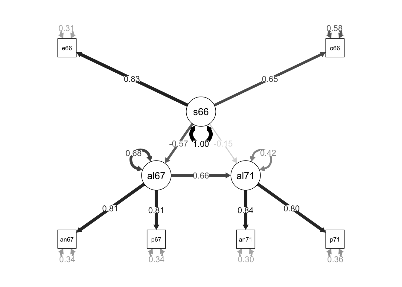
modificationindices(sem.fit)## lhs op rhs mi epc sepc.lv sepc.all sepc.nox
## 19 alien67 =~ anomia71 2.474 0.415 0.337 0.337 0.337
## 20 alien67 =~ pwless71 2.474 -0.394 -0.320 -0.321 -0.321
## 21 alien67 =~ educ66 0.223 -0.114 -0.093 -0.093 -0.093
## 22 alien67 =~ occstat66 0.223 0.089 0.072 0.072 0.072
## 23 alien71 =~ anomia67 3.491 0.292 0.245 0.246 0.246
## 24 alien71 =~ pwless67 3.491 -0.292 -0.245 -0.245 -0.245
## 25 alien71 =~ educ66 0.223 0.066 0.055 0.055 0.055
## 26 alien71 =~ occstat66 0.223 -0.051 -0.043 -0.043 -0.043
## 27 ses66 =~ anomia67 3.491 0.113 0.094 0.094 0.094
## 28 ses66 =~ pwless67 3.491 -0.113 -0.094 -0.094 -0.094
## 29 ses66 =~ anomia71 2.474 0.093 0.077 0.077 0.077
## 30 ses66 =~ pwless71 2.474 -0.088 -0.073 -0.073 -0.073
## 32 anomia67 ~~ anomia71 63.854 0.160 0.160 0.507 0.507
## 33 anomia67 ~~ pwless71 49.946 -0.139 -0.139 -0.395 -0.395
## 34 anomia67 ~~ educ66 6.069 0.052 0.052 0.161 0.161
## 35 anomia67 ~~ occstat66 1.261 -0.023 -0.023 -0.052 -0.052
## 36 pwless67 ~~ anomia71 49.929 -0.142 -0.142 -0.447 -0.447
## 37 pwless67 ~~ pwless71 37.398 0.120 0.120 0.341 0.341
## 38 pwless67 ~~ educ66 7.760 -0.059 -0.059 -0.181 -0.181
## 39 pwless67 ~~ occstat66 2.325 0.031 0.031 0.070 0.070
## 41 anomia71 ~~ educ66 3.631 0.039 0.039 0.130 0.130
## 42 anomia71 ~~ occstat66 0.547 -0.015 -0.015 -0.036 -0.036
## 43 pwless71 ~~ educ66 2.696 -0.033 -0.033 -0.099 -0.099
## 44 pwless71 ~~ occstat66 0.127 0.007 0.007 0.016 0.0163.0.3 Modifying our model
sem.model <- '
  # latent variable measurements
  alien67 =~ anomia67 + pwless67
  alien71 =~ anomia71 + pwless71
  ses66 =~ educ66 + occstat66

  # structural models
  alien67 ~ ses66
  alien71 ~ alien67 + ses66

  # residual correlations
  anomia67 ~~ anomia71
  pwless67 ~~ pwless71
'

sem.fit <- sem(sem.model, sample.cov = sem.data, sample.nobs = 933)
summary(sem.fit, standardized = TRUE)
## lavaan 0.6-9 ended normally after 30 iterations
##
## Estimator ML
## Optimization method NLMINB
## Number of model parameters 17
##
## Number of observations 933
##
## Model Test User Model:
##
## Test statistic 4.780
## Degrees of freedom 4
## P-value (Chi-square) 0.311
##
## Parameter Estimates:
##
## Standard errors Standard
## Information Expected
## Information saturated (h1) model Structured
##
## Latent Variables:
## Estimate Std.Err z-value P(>|z|) Std.lv Std.all
## alien67 =~
## anomia67 1.000 0.774 0.775
## pwless67 1.100 0.069 15.906 0.000 0.852 0.852
## alien71 =~
## anomia71 1.000 0.805 0.806
## pwless71 1.033 0.067 15.509 0.000 0.831 0.832
## ses66 =~
## educ66 1.000 0.841 0.841
## occstat66 0.763 0.062 12.373 0.000 0.641 0.642
##
## Regressions:
## Estimate Std.Err z-value P(>|z|) Std.lv Std.all
## alien67 ~
## ses66 -0.518 0.051 -10.203 0.000 -0.563 -0.563
## alien71 ~
## alien67 0.590 0.050 11.903 0.000 0.567 0.567
## ses66 -0.199 0.046 -4.339 0.000 -0.208 -0.208
##
## Covariances:
## Estimate Std.Err z-value P(>|z|) Std.lv Std.all
## .anomia67 ~~
## .anomia71 0.133 0.026 5.177 0.000 0.133 0.356
## .pwless67 ~~
## .pwless71 0.035 0.027 1.304 0.192 0.035 0.121
##
## Variances:
## Estimate Std.Err z-value P(>|z|) Std.lv Std.all
## .anomia67 0.400 0.038 10.443 0.000 0.400 0.400
## .pwless67 0.274 0.043 6.364 0.000 0.274 0.274
## .anomia71 0.351 0.041 8.540 0.000 0.351 0.351
## .pwless71 0.308 0.043 7.082 0.000 0.308 0.308
## .educ66 0.292 0.053 5.535 0.000 0.292 0.292
## .occstat66 0.587 0.040 14.602 0.000 0.587 0.588
## .alien67 0.409 0.039 10.366 0.000 0.683 0.683
## .alien71 0.326 0.032 10.110 0.000 0.503 0.503
## ses66 0.707 0.067 10.481 0.000 1.000 1.0003.0.4 Indirect effects
sem.model <- '
  # latent variable measurements
  alien67 =~ anomia67 + pwless67
  alien71 =~ anomia71 + pwless71
  ses66 =~ educ66 + occstat66

  # direct effects
  alien67 ~ b1 * ses66
  alien71 ~ a1 * alien67 + a2 * ses66

  # indirect effects
  ind := a1 * b1

  # total effect
  tot_eff := a1 * b1 + a2

  # residual correlations
  anomia67 ~~ anomia71
  pwless67 ~~ pwless71
'

sem.fit <- sem(sem.model, sample.cov = sem.data, sample.nobs = 933, std.lv = TRUE)
summary(sem.fit, standardized = TRUE)
## lavaan 0.6-9 ended normally after 30 iterations
##
## Estimator ML
## Optimization method NLMINB
## Number of model parameters 17
##
## Number of observations 933
##
## Model Test User Model:
##
## Test statistic 4.780
## Degrees of freedom 4
## P-value (Chi-square) 0.311
##
## Parameter Estimates:
##
## Standard errors Standard
## Information Expected
## Information saturated (h1) model Structured
##
## Latent Variables:
## Estimate Std.Err z-value P(>|z|) Std.lv Std.all
## alien67 =~
## anomia67 0.640 0.031 20.731 0.000 0.774 0.775
## pwless67 0.704 0.035 20.047 0.000 0.852 0.852
## alien71 =~
## anomia71 0.571 0.028 20.220 0.000 0.805 0.806
## pwless71 0.589 0.029 20.216 0.000 0.831 0.832
## ses66 =~
## educ66 0.841 0.040 20.962 0.000 0.841 0.841
## occstat66 0.641 0.037 17.242 0.000 0.641 0.642
##
## Regressions:
## Estimate Std.Err z-value P(>|z|) Std.lv Std.all
## alien67 ~
## ses66 (b1) -0.681 0.061 -11.121 0.000 -0.563 -0.563
## alien71 ~
## alien67 (a1) 0.661 0.064 10.282 0.000 0.567 0.567
## ses66 (a2) -0.293 0.065 -4.512 0.000 -0.208 -0.208
##
## Covariances:
## Estimate Std.Err z-value P(>|z|) Std.lv Std.all
## .anomia67 ~~
## .anomia71 0.133 0.026 5.177 0.000 0.133 0.356
## .pwless67 ~~
## .pwless71 0.035 0.027 1.304 0.192 0.035 0.121
##
## Variances:
## Estimate Std.Err z-value P(>|z|) Std.lv Std.all
## .anomia67 0.400 0.038 10.443 0.000 0.400 0.400
## .pwless67 0.274 0.043 6.364 0.000 0.274 0.274
## .anomia71 0.351 0.041 8.540 0.000 0.351 0.351
## .pwless71 0.308 0.043 7.082 0.000 0.308 0.308
## .educ66 0.292 0.053 5.535 0.000 0.292 0.292
## .occstat66 0.587 0.040 14.602 0.000 0.587 0.588
## .alien67 1.000 0.683 0.683
## .alien71 1.000 0.503 0.503
## ses66 1.000 1.000 1.000
##
## Defined Parameters:
## Estimate Std.Err z-value P(>|z|) Std.lv Std.all
## ind -0.450 0.051 -8.895 0.000 -0.319 -0.319
## tot_eff -0.743 0.066 -11.285 0.000 -0.527 -0.5273.1 Equality constraints
- when the same conceptual variable appears more than once as a latent variable in a model, we should consider using equality constraints
- before we can say that alienation in 1967 and alienation in 1971 are measuring the same concept we need to establish the equivalence of the measurement of alienation
- with SEM we can test whether indicators have the same factor loadings across latent variables. This is what invariance is
- first level requires the same set of indicators be relevant to the latent variable
- the first level allows the loadings and the error variances for the observed measures to vary from one wave to the next
- second level adds the requirement that some of the indicators have the same loadings and other differ only by a fairly small amount
- third level adds that the loadings be invariant but allows the error variances to be free
- fourth level is when the loadings and the error variances are invariant across waves
- first level requires the same set of indicators be relevant to the latent variable
3.2 Programming constraints
- we want to compare estimates from the unstandardized model
sem.model <- '
  # latent variable measurements
  alien67 =~ anomia67 + pwless67
  alien71 =~ anomia71 + pwless71
  ses66 =~ educ66 + occstat66

  # direct effects
  alien67 ~ b1 * ses66
  alien71 ~ a1 * alien67 + a2 * ses66

  # indirect effects
  ind := a1 * b1

  # total effect
  tot_eff := a1 * b1 + a2

  # residual correlations
  anomia67 ~~ anomia71
  pwless67 ~~ pwless71
'

sem.fit <- sem(sem.model, sample.cov = sem.data, sample.nobs = 933,
               meanstructure = TRUE, std.lv = TRUE)
summary(sem.fit)
## lavaan 0.6-9 ended normally after 30 iterations
##
## Estimator ML
## Optimization method NLMINB
## Number of model parameters 23
##
## Number of observations 933
##
## Model Test User Model:
##
## Test statistic 4.780
## Degrees of freedom 4
## P-value (Chi-square) 0.311
##
## Parameter Estimates:
##
## Standard errors Standard
## Information Expected
## Information saturated (h1) model Structured
##
## Latent Variables:
## Estimate Std.Err z-value P(>|z|)
## alien67 =~
## anomia67 0.640 0.031 20.731 0.000
## pwless67 0.704 0.035 20.047 0.000
## alien71 =~
## anomia71 0.571 0.028 20.220 0.000
## pwless71 0.589 0.029 20.216 0.000
## ses66 =~
## educ66 0.841 0.040 20.962 0.000
## occstat66 0.641 0.037 17.242 0.000
##
## Regressions:
## Estimate Std.Err z-value P(>|z|)
## alien67 ~
## ses66 (b1) -0.681 0.061 -11.121 0.000
## alien71 ~
## alien67 (a1) 0.661 0.064 10.282 0.000
## ses66 (a2) -0.293 0.065 -4.512 0.000
##
## Covariances:
## Estimate Std.Err z-value P(>|z|)
## .anomia67 ~~
## .anomia71 0.133 0.026 5.177 0.000
## .pwless67 ~~
## .pwless71 0.035 0.027 1.304 0.192
##
## Intercepts:
## Estimate Std.Err z-value P(>|z|)
## .anomia67 0.000 0.033 0.000 1.000
## .pwless67 0.000 0.033 0.000 1.000
## .anomia71 0.000 0.033 0.000 1.000
## .pwless71 0.000 0.033 0.000 1.000
## .educ66 0.000 0.033 0.000 1.000
## .occstat66 0.000 0.033 0.000 1.000
## .alien67 0.000
## .alien71 0.000
## ses66 0.000
##
## Variances:
## Estimate Std.Err z-value P(>|z|)
## .anomia67 0.400 0.038 10.443 0.000
## .pwless67 0.274 0.043 6.364 0.000
## .anomia71 0.351 0.041 8.540 0.000
## .pwless71 0.308 0.043 7.082 0.000
## .educ66 0.292 0.053 5.535 0.000
## .occstat66 0.587 0.040 14.602 0.000
## .alien67 1.000
## .alien71 1.000
## ses66 1.000
##
## Defined Parameters:
## Estimate Std.Err z-value P(>|z|)
## ind -0.450 0.051 -8.895 0.000
## tot_eff -0.743 0.066 -11.285 0.000if all loadings are significant, then we meet the first level of invariance
to test for additional levels of invariance, we need to check for equivalance of loadings for
pwless67andpwless71
sem.model <- '
  # latent variable measurements
  alien67 =~ anomia67 + l1 * pwless67
  alien71 =~ anomia71 + l1 * pwless71
  ses66 =~ educ66 + occstat66

  # direct effects
  alien67 ~ b1 * ses66
  alien71 ~ a1 * alien67 + a2 * ses66

  # indirect effects
  ind := a1 * b1

  # total effect
  tot_eff := a1 * b1 + a2

  # residual correlations
  anomia67 ~~ anomia71
  pwless67 ~~ pwless71
'

sem.fit <- sem(sem.model, sample.cov = sem.data, sample.nobs = 933,
               std.lv = TRUE)
summary(sem.fit)
## lavaan 0.6-9 ended normally after 28 iterations
##
## Estimator ML
## Optimization method NLMINB
## Number of model parameters 17
## Number of equality constraints 1
##
## Number of observations 933
##
## Model Test User Model:
##
## Test statistic 12.722
## Degrees of freedom 5
## P-value (Chi-square) 0.026
##
## Parameter Estimates:
##
## Standard errors Standard
## Information Expected
## Information saturated (h1) model Structured
##
## Latent Variables:
## Estimate Std.Err z-value P(>|z|)
## alien67 =~
## anomia67 0.612 0.029 21.142 0.000
## pwless67 (l1) 0.640 0.025 25.679 0.000
## alien71 =~
## anomia71 0.591 0.027 21.584 0.000
## pwless71 (l1) 0.640 0.025 25.679 0.000
## ses66 =~
## educ66 0.827 0.039 21.389 0.000
## occstat66 0.647 0.037 17.678 0.000
##
## Regressions:
## Estimate Std.Err z-value P(>|z|)
## alien67 ~
## ses66 (b1) -0.756 0.060 -12.522 0.000
## alien71 ~
## alien67 (a1) 0.581 0.056 10.301 0.000
## ses66 (a2) -0.271 0.067 -4.028 0.000
##
## Covariances:
## Estimate Std.Err z-value P(>|z|)
## .anomia67 ~~
## .anomia71 0.135 0.025 5.478 0.000
## .pwless67 ~~
## .pwless71 0.040 0.026 1.556 0.120
##
## Variances:
## Estimate Std.Err z-value P(>|z|)
## .anomia67 0.383 0.037 10.462 0.000
## .pwless67 0.309 0.037 8.265 0.000
## .anomia71 0.368 0.041 8.971 0.000
## .pwless71 0.278 0.045 6.140 0.000
## .educ66 0.314 0.049 6.439 0.000
## .occstat66 0.580 0.039 14.745 0.000
## .alien67 1.000
## .alien71 1.000
## ses66 1.000
##
## Defined Parameters:
## Estimate Std.Err z-value P(>|z|)
## ind -0.439 0.052 -8.499 0.000
## tot_eff -0.710 0.061 -11.562 0.0003.3 Structural model with formative indicators
reflective indicators are where the latent variable causes the response on the observed variable
formative indicators are where the latent variable is caused by the observed variable
3.3.1 Identification and estimation of a composite latent variable
sem.model <- '
  # latent variable measurements
  alien67 =~ anomia67 + l1 * pwless67
  alien71 =~ anomia71 + l1 * pwless71
  ses66 <~ 1 * educ66 + occstat66 # formative indicators

  # direct effects
  alien67 ~ b1 * ses66
  alien71 ~ a1 * alien67 + a2 * ses66

  # indirect effects
  ind := a1 * b1

  # total effect
  tot_eff := a1 * b1 + a2

  # residual correlations
  anomia67 ~~ anomia71
  pwless67 ~~ pwless71
'

sem.fit <- sem(sem.model, sample.cov = sem.data, sample.nobs = 932)
summary(sem.fit, standardized = TRUE)
## lavaan 0.6-9 ended normally after 28 iterations
##
## Estimator ML
## Optimization method NLMINB
## Number of model parameters 14
## Number of equality constraints 1
##
## Number of observations 932
##
## Model Test User Model:
##
## Test statistic 5.772
## Degrees of freedom 5
## P-value (Chi-square) 0.329
##
## Parameter Estimates:
##
## Standard errors Standard
## Information Expected
## Information saturated (h1) model Structured
##
## Latent Variables:
## Estimate Std.Err z-value P(>|z|) Std.lv Std.all
## alien67 =~
## anomia67 1.000 0.785 0.783
## pwless67 (l1) 1.068 0.059 18.138 0.000 0.839 0.842
## alien71 =~
## anomia71 1.000 0.792 0.795
## pwless71 (l1) 1.068 0.059 18.138 0.000 0.846 0.843
##
## Composites:
## Estimate Std.Err z-value P(>|z|) Std.lv Std.all
## ses66 <~
## educ66 1.000 0.802 0.801
## occstat66 0.381 0.111 3.425 0.001 0.306 0.305
##
## Regressions:
## Estimate Std.Err z-value P(>|z|) Std.lv Std.all
## alien67 ~
## ses66 (b1) -0.309 0.031 -9.961 0.000 -0.491 -0.491
## alien71 ~
## alien67 (a1) 0.611 0.041 15.055 0.000 0.606 0.606
## ses66 (a2) -0.102 0.023 -4.361 0.000 -0.161 -0.161
##
## Covariances:
## Estimate Std.Err z-value P(>|z|) Std.lv Std.all
## .anomia67 ~~
## .anomia71 0.134 0.026 5.197 0.000 0.134 0.355
## .pwless67 ~~
## .pwless71 0.034 0.027 1.256 0.209 0.034 0.117
##
## Variances:
## Estimate Std.Err z-value P(>|z|) Std.lv Std.all
## .anomia67 0.389 0.037 10.425 0.000 0.389 0.387
## .pwless67 0.288 0.040 7.227 0.000 0.288 0.290
## .anomia71 0.365 0.038 9.601 0.000 0.365 0.367
## .pwless71 0.291 0.041 7.062 0.000 0.291 0.289
## .alien67 0.468 0.040 11.844 0.000 0.759 0.759
## .alien71 0.321 0.030 10.838 0.000 0.512 0.512
## ses66 0.000 0.000 0.000
##
## Defined Parameters:
## Estimate Std.Err z-value P(>|z|) Std.lv Std.all
## ind -0.189 0.023 -8.307 0.000 -0.297 -0.297
## tot_eff -0.291 0.030 -9.618 0.000 -0.458 -0.4583.3.2 Multiple indicators, multiple causes model
when we fix the error variance of
ses66to 0 and the unstandardized coefficient fromeduc66toses66at 1 it means that our latent variable is assumed to be a perfect composite of the observed formative indicatorsa multiple indicators, multiple causes model allows us to have a nonzero variance