Chapter 2 Using structural equation modeling for path models
2.1 A substantive example of a path model
library(haven)

path.data <- read_dta("path.dta")

# path model
library(lavaan)

path.model <- '
  # direct effects
  math21 ~ a1 * attention4 + a2 * math7 + a3 * read7
  math7 ~ b1 * attention4
  read7 ~ c1 * attention4

  # indirect effects
  ind1 := b1 * a2
  ind2 := c1 * a3
'

path.fit <- sem(path.model, estimator = "ML", data = path.data)
summary(path.fit, fit.measures = TRUE, rsquare =  TRUE)
## lavaan 0.6-9 ended normally after 22 iterations
##
## Estimator ML
## Optimization method NLMINB
## Number of model parameters 8
##
## Used Total
## Number of observations 338 430
##
## Model Test User Model:
##
## Test statistic 23.725
## Degrees of freedom 1
## P-value (Chi-square) 0.000
##
## Model Test Baseline Model:
##
## Test statistic 118.786
## Degrees of freedom 6
## P-value 0.000
##
## User Model versus Baseline Model:
##
## Comparative Fit Index (CFI) 0.799
## Tucker-Lewis Index (TLI) -0.209
##
## Loglikelihood and Information Criteria:
##
## Loglikelihood user model (H0) -2788.235
## Loglikelihood unrestricted model (H1) -2776.372
##
## Akaike (AIC) 5592.469
## Bayesian (BIC) 5623.053
## Sample-size adjusted Bayesian (BIC) 5597.676
##
## Root Mean Square Error of Approximation:
##
## RMSEA 0.259
## 90 Percent confidence interval - lower 0.175
## 90 Percent confidence interval - upper 0.354
## P-value RMSEA <= 0.05 0.000
##
## Standardized Root Mean Square Residual:
##
## SRMR 0.088
##
## Parameter Estimates:
##
## Standard errors Standard
## Information Expected
## Information saturated (h1) model Structured
##
## Regressions:
## Estimate Std.Err z-value P(>|z|)
## math21 ~
## attentin4 (a1) 0.081 0.042 1.927 0.054
## math7 (a2) 0.294 0.046 6.399 0.000
## read7 (a3) 0.083 0.016 5.253 0.000
## math7 ~
## attentin4 (b1) 0.113 0.049 2.290 0.022
## read7 ~
## attentin4 (c1) 0.302 0.144 2.098 0.036
##
## Variances:
## Estimate Std.Err z-value P(>|z|)
## .math21 5.590 0.430 13.000 0.000
## .math7 7.842 0.603 13.000 0.000
## .read7 66.979 5.152 13.000 0.000
##
## R-Square:
## Estimate
## math21 0.191
## math7 0.015
## read7 0.013
##
## Defined Parameters:
## Estimate Std.Err z-value P(>|z|)
## ind1 0.033 0.015 2.156 0.031
## ind2 0.025 0.013 1.949 0.051library(broom)
tidy(path.fit)## # A tibble: 11 × 10
## term op label estimate std.error statistic p.value std.lv std.all
## <chr> <chr> <chr> <dbl> <dbl> <dbl> <dbl> <dbl> <dbl>
## 1 math21 ~ … ~ "a1" 0.0814 0.0422 1.93 5.40e- 2 0.0814 0.0956
## 2 math21 ~ … ~ "a2" 0.294 0.0459 6.40 1.57e-10 0.294 0.315
## 3 math21 ~ … ~ "a3" 0.0825 0.0157 5.25 1.50e- 7 0.0825 0.259
## 4 math7 ~ a… ~ "b1" 0.113 0.0493 2.29 2.20e- 2 0.113 0.124
## 5 read7 ~ a… ~ "c1" 0.302 0.144 2.10 3.59e- 2 0.302 0.113
## 6 math21 ~~… ~~ "" 5.59 0.430 13 0 5.59 0.809
## 7 math7 ~~ … ~~ "" 7.84 0.603 13.0 0 7.84 0.985
## 8 read7 ~~ … ~~ "" 67.0 5.15 13 0 67.0 0.987
## 9 attention… ~~ "" 9.54 0 NA NA 9.54 1
## 10 ind1 := b… := "ind… 0.0332 0.0154 2.16 3.11e- 2 0.0332 0.0390
## 11 ind2 := c… := "ind… 0.0250 0.0128 1.95 5.13e- 2 0.0250 0.0293
## # … with 1 more variable: std.nox <dbl>library(lavaanPlot)
lavaanPlot(model = path.fit, coefs = TRUE, stand = TRUE)library(semPlot)
semPaths(object = path.fit, what = "std", edge.label.cex = 1, curvePivot = TRUE,
fixedStyle = c("black", 1), freeStyle = c("black", 1),
edge.color = "black")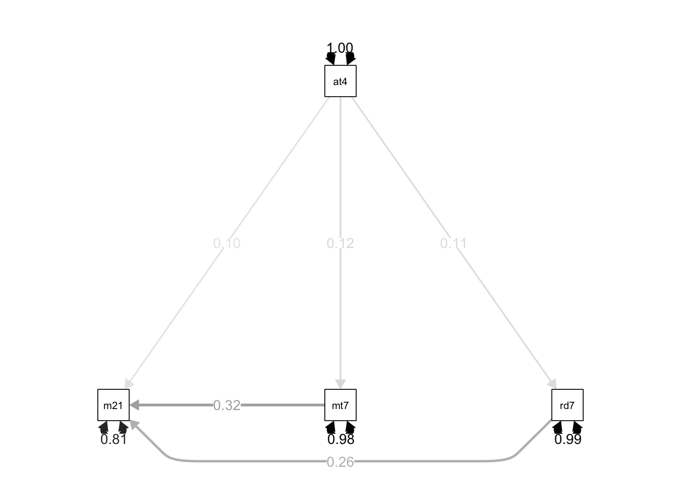
- with SEM a significant chi-squared means that we fail to account for the covariances among our variables
2.2 Estimating a model with correlated residuals
- we add a residual correlation between
read7andmath7. This says that there are variables excluded in the model that influence both of these variables
path.model <- '
  # direct effects
  math21 ~ a1 * attention4 + a2 * math7 + a3 * read7
  math7 ~ b1 * attention4
  read7 ~ c1 * attention4

  # indirect effects
  ind1 := b1 * a2
  ind2 := c1 * a3

  # total effects
  total_att := a1 + a2 * b1

  # residual correlations
  math7 ~~ read7
'

path.fit <- sem(path.model, data = path.data)
summary(path.fit, fit.measures = TRUE, rsquare =  TRUE)
## lavaan 0.6-9 ended normally after 32 iterations
##
## Estimator ML
## Optimization method NLMINB
## Number of model parameters 9
##
## Used Total
## Number of observations 338 430
##
## Model Test User Model:
##
## Test statistic 0.000
## Degrees of freedom 0
##
## Model Test Baseline Model:
##
## Test statistic 118.786
## Degrees of freedom 6
## P-value 0.000
##
## User Model versus Baseline Model:
##
## Comparative Fit Index (CFI) 1.000
## Tucker-Lewis Index (TLI) 1.000
##
## Loglikelihood and Information Criteria:
##
## Loglikelihood user model (H0) -2776.372
## Loglikelihood unrestricted model (H1) -2776.372
##
## Akaike (AIC) 5570.744
## Bayesian (BIC) 5605.152
## Sample-size adjusted Bayesian (BIC) 5576.602
##
## Root Mean Square Error of Approximation:
##
## RMSEA 0.000
## 90 Percent confidence interval - lower 0.000
## 90 Percent confidence interval - upper 0.000
## P-value RMSEA <= 0.05 NA
##
## Standardized Root Mean Square Residual:
##
## SRMR 0.000
##
## Parameter Estimates:
##
## Standard errors Standard
## Information Expected
## Information saturated (h1) model Structured
##
## Regressions:
## Estimate Std.Err z-value P(>|z|)
## math21 ~
## attentin4 (a1) 0.081 0.042 1.932 0.053
## math7 (a2) 0.294 0.048 6.178 0.000
## read7 (a3) 0.083 0.016 5.072 0.000
## math7 ~
## attentin4 (b1) 0.113 0.049 2.290 0.022
## read7 ~
## attentin4 (c1) 0.302 0.144 2.098 0.036
##
## Covariances:
## Estimate Std.Err z-value P(>|z|)
## .math7 ~~
## .read7 5.967 1.288 4.632 0.000
##
## Variances:
## Estimate Std.Err z-value P(>|z|)
## .math21 5.590 0.430 13.000 0.000
## .math7 7.842 0.603 13.000 0.000
## .read7 66.979 5.152 13.000 0.000
##
## R-Square:
## Estimate
## math21 0.223
## math7 0.015
## read7 0.013
##
## Defined Parameters:
## Estimate Std.Err z-value P(>|z|)
## ind1 0.033 0.015 2.147 0.032
## ind2 0.025 0.013 1.939 0.053
## total_att 0.115 0.044 2.582 0.010tidy(path.fit)## # A tibble: 13 × 10
## term op label estimate std.error statistic p.value std.lv std.all
## <chr> <chr> <chr> <dbl> <dbl> <dbl> <dbl> <dbl> <dbl>
## 1 math21 ~… ~ "a1" 0.0814 0.0421 1.93 5.33e- 2 0.0814 0.0937
## 2 math21 ~… ~ "a2" 0.294 0.0476 6.18 6.49e-10 0.294 0.309
## 3 math21 ~… ~ "a3" 0.0825 0.0163 5.07 3.94e- 7 0.0825 0.253
## 4 math7 ~ … ~ "b1" 0.113 0.0493 2.29 2.20e- 2 0.113 0.124
## 5 read7 ~ … ~ "c1" 0.302 0.144 2.10 3.59e- 2 0.302 0.113
## 6 math7 ~~… ~~ "" 5.97 1.29 4.63 3.62e- 6 5.97 0.260
## 7 math21 ~… ~~ "" 5.59 0.430 13 0 5.59 0.777
## 8 math7 ~~… ~~ "" 7.84 0.603 13.0 0 7.84 0.985
## 9 read7 ~~… ~~ "" 67.0 5.15 13 0 67.0 0.987
## 10 attentio… ~~ "" 9.54 0 NA NA 9.54 1
## 11 ind1 := … := "ind1" 0.0332 0.0155 2.15 3.18e- 2 0.0332 0.0382
## 12 ind2 := … := "ind2" 0.0250 0.0129 1.94 5.25e- 2 0.0250 0.0287
## 13 total_at… := "tota… 0.115 0.0444 2.58 9.82e- 3 0.115 0.132
## # … with 1 more variable: std.nox <dbl>semPaths(object = path.fit, what = "std", edge.label.cex = 1, curvePivot = TRUE,
fixedStyle = c("black", 1), freeStyle = c("black", 1),
edge.color = "black")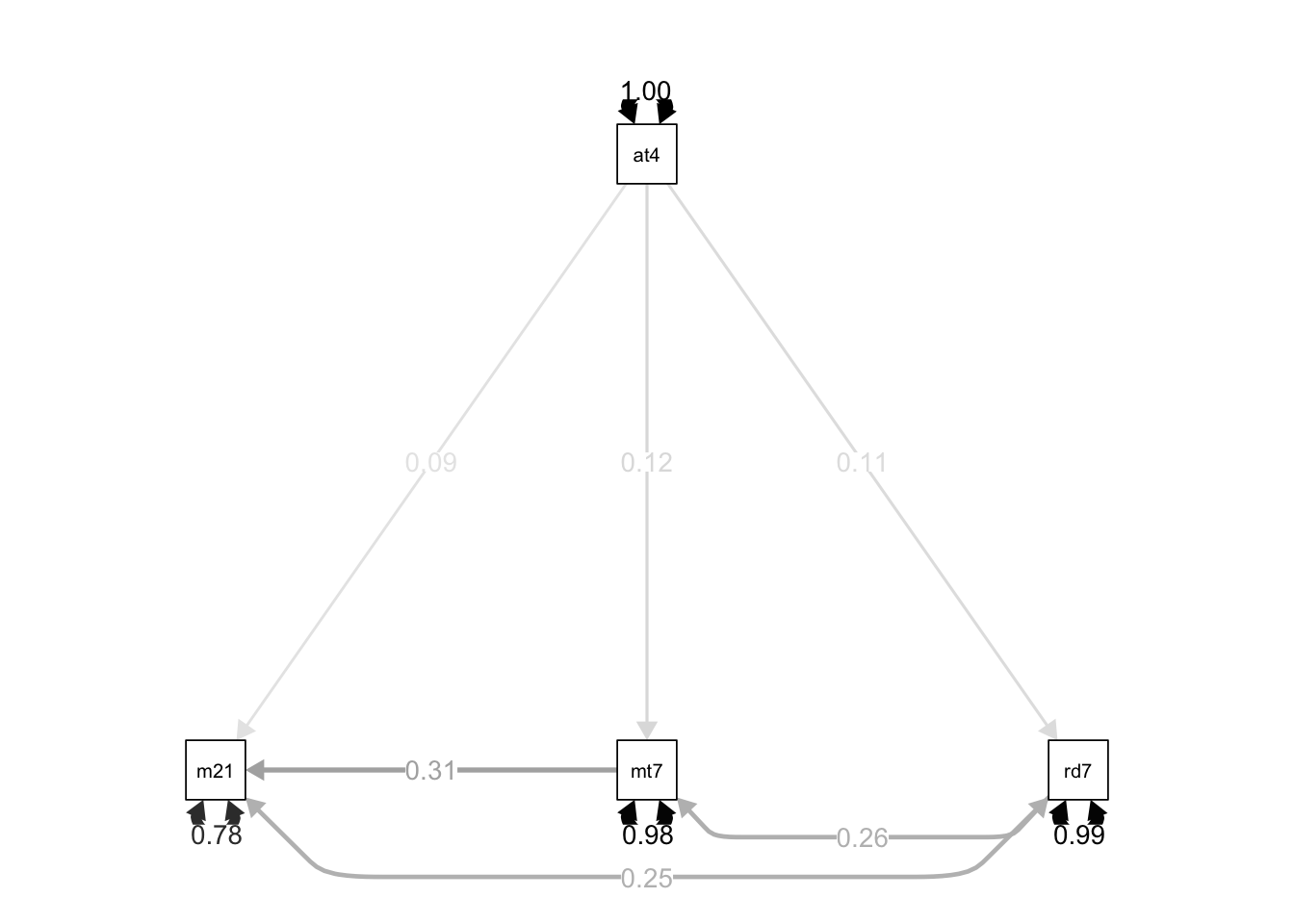
2.2.1 Strengthening our path model and adding covariates
path.model <- '
  # direct effects
  math21 ~ a1 * attention4 + a2 * math7 + a3 * read7 + vocab4 + adopted + male
    + momed
  math7 ~ b1 * attention4 + vocab4 + adopted + male + momed
  read7 ~ c1 * attention4 + vocab4 + adopted + male + momed

  # indirect effects
  ind1 := b1 * a2
  ind2 := c1 * a3

  # total effects
  total_att := a1 + a2 * b1

  # residual correlations
  math7 ~~ read7
'

path.fit <- sem(path.model, estimator = "MLMV", data = path.data)
summary(path.fit, fit.measures = TRUE, rsquare =  TRUE)
## lavaan 0.6-9 ended normally after 77 iterations
##
## Estimator ML
## Optimization method NLMINB
## Number of model parameters 21
##
## Used Total
## Number of observations 299 430
##
## Model Test User Model:
## Standard Robust
## Test Statistic 0.000 0.000
## Degrees of freedom 0 0
##
## Model Test Baseline Model:
##
## Test statistic 158.786 146.884
## Degrees of freedom 18 18
## P-value 0.000 0.000
## Scaling correction factor 1.101
##
## User Model versus Baseline Model:
##
## Comparative Fit Index (CFI) 1.000 1.000
## Tucker-Lewis Index (TLI) 1.000 1.000
##
## Robust Comparative Fit Index (CFI) NA
## Robust Tucker-Lewis Index (TLI) NA
##
## Loglikelihood and Information Criteria:
##
## Loglikelihood user model (H0) -2424.712 -2424.712
## Loglikelihood unrestricted model (H1) -2424.712 -2424.712
##
## Akaike (AIC) 4891.424 4891.424
## Bayesian (BIC) 4969.133 4969.133
## Sample-size adjusted Bayesian (BIC) 4902.534 4902.534
##
## Root Mean Square Error of Approximation:
##
## RMSEA 0.000 0.000
## 90 Percent confidence interval - lower 0.000 0.000
## 90 Percent confidence interval - upper 0.000 0.000
## P-value RMSEA <= 0.05 NA NA
##
## Robust RMSEA NA
## 90 Percent confidence interval - lower 0.000
## 90 Percent confidence interval - upper 0.000
##
## Standardized Root Mean Square Residual:
##
## SRMR 0.000 0.000
##
## Parameter Estimates:
##
## Standard errors Robust.sem
## Information Expected
## Information saturated (h1) model Structured
##
## Regressions:
## Estimate Std.Err z-value P(>|z|)
## math21 ~
## attentin4 (a1) 0.064 0.044 1.458 0.145
## math7 (a2) 0.272 0.048 5.653 0.000
## read7 (a3) 0.078 0.017 4.615 0.000
## vocab4 -0.022 0.053 -0.424 0.671
## adopted -0.779 0.269 -2.889 0.004
## male 1.224 0.265 4.624 0.000
## momed -0.036 0.068 -0.527 0.598
## math7 ~
## attentin4 (b1) 0.065 0.051 1.267 0.205
## vocab4 0.250 0.066 3.772 0.000
## adopted -0.688 0.311 -2.213 0.027
## male -0.254 0.311 -0.814 0.415
## momed -0.083 0.075 -1.106 0.269
## read7 ~
## attentin4 (c1) 0.286 0.149 1.920 0.055
## vocab4 0.431 0.194 2.227 0.026
## adopted -0.272 0.931 -0.292 0.771
## male 0.336 0.930 0.362 0.718
## momed 0.463 0.234 1.981 0.048
##
## Covariances:
## Estimate Std.Err z-value P(>|z|)
## .math7 ~~
## .read7 5.716 1.224 4.668 0.000
##
## Variances:
## Estimate Std.Err z-value P(>|z|)
## .math21 5.028 0.436 11.525 0.000
## .math7 7.219 0.534 13.510 0.000
## .read7 65.680 5.719 11.485 0.000
##
## R-Square:
## Estimate
## math21 0.278
## math7 0.079
## read7 0.050
##
## Defined Parameters:
## Estimate Std.Err z-value P(>|z|)
## ind1 0.018 0.014 1.247 0.213
## ind2 0.022 0.012 1.780 0.075
## total_att 0.082 0.048 1.701 0.089tidy(path.fit)## # A tibble: 39 × 10
## term op label estimate std.error statistic p.value std.lv std.all
## <chr> <chr> <chr> <dbl> <dbl> <dbl> <dbl> <dbl> <dbl>
## 1 math21 ~ a… ~ "a1" 0.0638 0.0438 1.46 1.45e-1 0.0638 0.0753
## 2 math21 ~ m… ~ "a2" 0.272 0.0482 5.65 1.57e-8 0.272 0.289
## 3 math21 ~ r… ~ "a3" 0.0775 0.0168 4.61 3.94e-6 0.0775 0.244
## 4 math21 ~ v… ~ "" -0.0223 0.0527 -0.424 6.71e-1 -0.0223 -0.0214
## 5 math21 ~ a… ~ "" -0.779 0.269 -2.89 3.86e-3 -0.779 -0.147
## 6 math21 ~ m… ~ "" 1.22 0.265 4.62 3.76e-6 1.22 0.231
## 7 math21 ~ m… ~ "" -0.0360 0.0683 -0.527 5.98e-1 -0.0360 -0.0268
## 8 math7 ~ at… ~ "b1" 0.0649 0.0512 1.27 2.05e-1 0.0649 0.0722
## 9 math7 ~ vo… ~ "" 0.250 0.0663 3.77 1.62e-4 0.250 0.226
## 10 math7 ~ ad… ~ "" -0.688 0.311 -2.21 2.69e-2 -0.688 -0.123
## # … with 29 more rows, and 1 more variable: std.nox <dbl>semPaths(object = path.fit, what = "std", edge.label.cex = 1, curvePivot = TRUE,
fixedStyle = c("black", 1), freeStyle = c("black", 1),
edge.color = "black")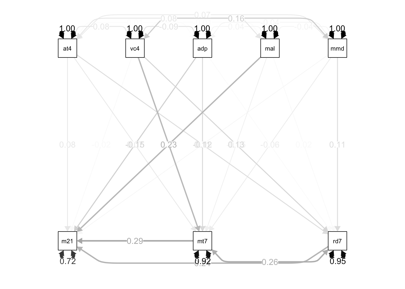
2.3 Auxiliary Variables
- an auxiliary variable is a variable that explains who is more likely to have missing values
path.model <- '
  # direct effects
  math21 ~ a1 * attention4 + a2 * math7 + a3 * read7 + vocab4 + adopted + male
    + momed
  math7 ~ b1 * attention4 + vocab4 + adopted + male + momed
  read7 ~ c1 * attention4 + vocab4 + adopted + male + momed

  # indirect effects
  ind1 := b1 * a2
  ind2 := c1 * a3

  # total effects
  total_att := a1 + a2 * b1

  # residual correlations
  math7 ~~ read7
'

library(semTools)
## ## ################################################################################# This is semTools 0.5-5## All users of R (or SEM) are invited to submit functions or ideas for functions.## #################################################################################
## Attaching package: 'semTools'## The following objects are masked from 'package:psych':
##
## reliability, skew## The following object is masked from 'package:readr':
##
## clipboard# path.fit <- sem.auxiliary(path.model, aux = "VAR HERE", data = path.data)2.4 Testing equality of coefficients
2.5 A cross-lagged panel design
suppose we want to know the influence of math scores on reading skills and the influence of reading skills on math scores
we can test this with panel data where we have a least two waves of data
path.model <- '
  # direct effects
  math21 ~ math7 + read7
  read21 ~ math7 + read7

  # residual correlations
  math7 ~~ read7
  math21 ~~ read21
'

path.fit <- sem(path.model, data = path.data)
summary(path.fit, fit.measures = TRUE, rsquare =  TRUE)
## lavaan 0.6-9 ended normally after 40 iterations
##
## Estimator ML
## Optimization method NLMINB
## Number of model parameters 10
##
## Used Total
## Number of observations 336 430
##
## Model Test User Model:
##
## Test statistic 0.000
## Degrees of freedom 0
##
## Model Test Baseline Model:
##
## Test statistic 236.276
## Degrees of freedom 6
## P-value 0.000
##
## User Model versus Baseline Model:
##
## Comparative Fit Index (CFI) 1.000
## Tucker-Lewis Index (TLI) 1.000
##
## Loglikelihood and Information Criteria:
##
## Loglikelihood user model (H0) -3895.659
## Loglikelihood unrestricted model (H1) -3895.659
##
## Akaike (AIC) 7811.319
## Bayesian (BIC) 7849.490
## Sample-size adjusted Bayesian (BIC) 7817.769
##
## Root Mean Square Error of Approximation:
##
## RMSEA 0.000
## 90 Percent confidence interval - lower 0.000
## 90 Percent confidence interval - upper 0.000
## P-value RMSEA <= 0.05 NA
##
## Standardized Root Mean Square Residual:
##
## SRMR 0.000
##
## Parameter Estimates:
##
## Standard errors Standard
## Information Expected
## Information saturated (h1) model Structured
##
## Regressions:
## Estimate Std.Err z-value P(>|z|)
## math21 ~
## math7 0.305 0.048 6.389 0.000
## read7 0.085 0.016 5.212 0.000
## read21 ~
## math7 0.353 0.142 2.487 0.013
## read7 0.510 0.049 10.495 0.000
##
## Covariances:
## Estimate Std.Err z-value P(>|z|)
## math7 ~~
## read7 6.295 1.318 4.776 0.000
## .math21 ~~
## .read21 3.090 0.934 3.308 0.001
##
## Variances:
## Estimate Std.Err z-value P(>|z|)
## .math21 5.668 0.437 12.961 0.000
## .read21 50.046 3.861 12.961 0.000
## math7 7.992 0.617 12.961 0.000
## read7 68.068 5.252 12.961 0.000
##
## R-Square:
## Estimate
## math21 0.216
## read21 0.295tidy(path.fit)## # A tibble: 10 × 9
## term op estimate std.error statistic p.value std.lv std.all std.nox
## <chr> <chr> <dbl> <dbl> <dbl> <dbl> <dbl> <dbl> <dbl>
## 1 math21 ~… ~ 0.305 0.0477 6.39 1.67e-10 0.305 0.320 0.320
## 2 math21 ~… ~ 0.0852 0.0163 5.21 1.87e- 7 0.0852 0.261 0.261
## 3 read21 ~… ~ 0.353 0.142 2.49 1.29e- 2 0.353 0.118 0.118
## 4 read21 ~… ~ 0.510 0.0486 10.5 0 0.510 0.499 0.499
## 5 math7 ~~… ~~ 6.30 1.32 4.78 1.79e- 6 6.30 0.270 0.270
## 6 math21 ~… ~~ 3.09 0.934 3.31 9.41e- 4 3.09 0.183 0.183
## 7 math21 ~… ~~ 5.67 0.437 13.0 0 5.67 0.784 0.784
## 8 read21 ~… ~~ 50.0 3.86 13.0 0 50.0 0.705 0.705
## 9 math7 ~~… ~~ 7.99 0.617 13.0 0 7.99 1 1
## 10 read7 ~~… ~~ 68.1 5.25 13.0 0 68.1 1 1semPaths(object = path.fit, what = "std", edge.label.cex = 1, curvePivot = TRUE,
fixedStyle = c("black", 1), freeStyle = c("black", 1),
edge.color = "black")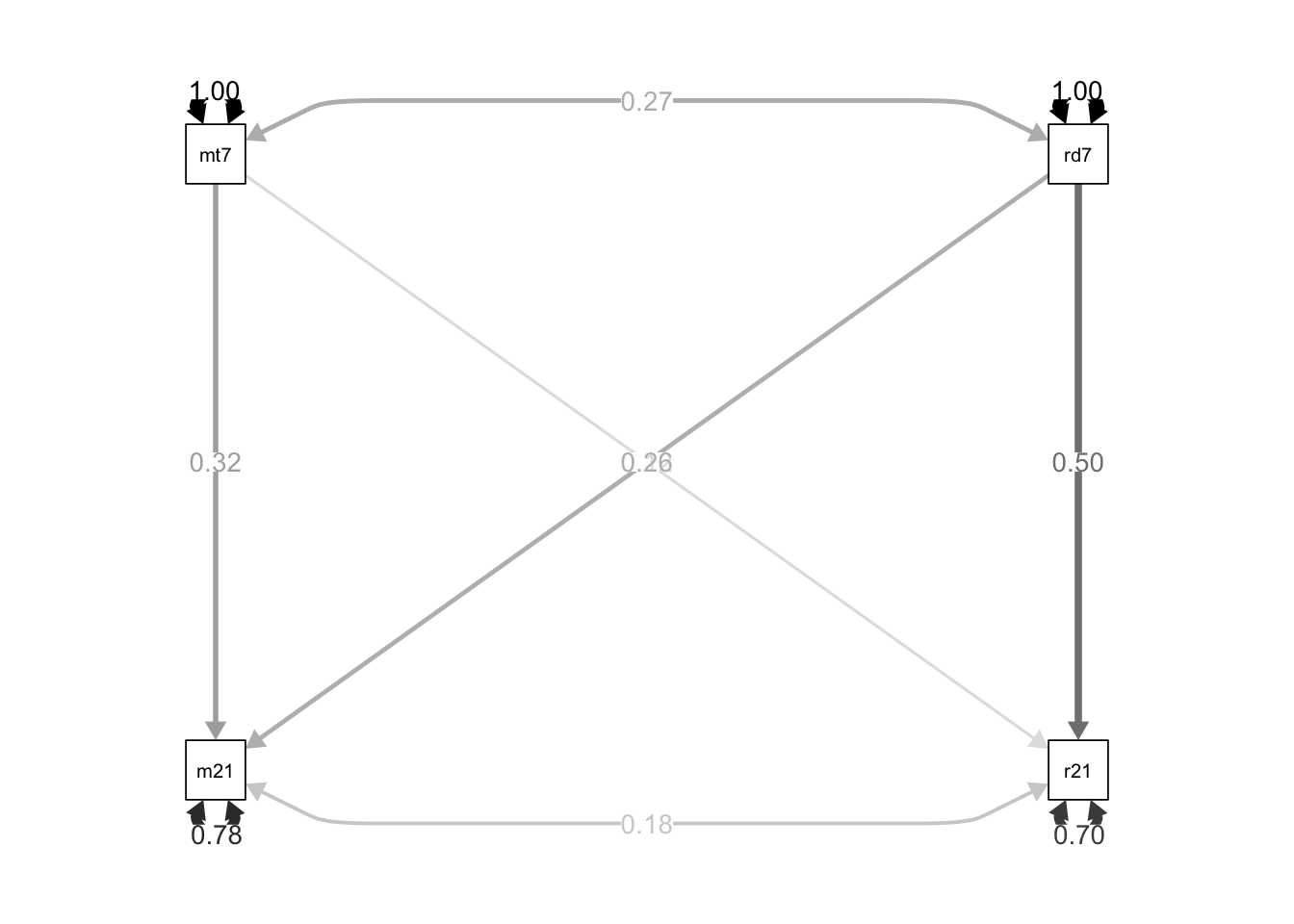
reading skills are more stable than math skills
reading skills are age 7 influence math skills are age 21 more than math skills at age 7 influence reading skills at age 21
2.6 Moderation
auto.data <- read_dta("auto.dta")

library(tidyverse)
auto.data <-
  auto.data %>%
  mutate(wgt1000s = weight / 1000)

path.model <- '
  mpg ~ wgt1000s
'

path.fit <- sem(path.model, data = auto.data)
tidy(path.fit)
## # A tibble: 3 × 9
## term op estimate std.error statistic p.value std.lv std.all std.nox
## <chr> <chr> <dbl> <dbl> <dbl> <dbl> <dbl> <dbl> <dbl>
## 1 mpg ~ wgt1… ~ -6.01 0.511 -11.8 0 -6.01 -0.807 -1.05
## 2 mpg ~~ mpg ~~ 11.5 1.89 6.08 1.18e-9 11.5 0.348 0.348
## 3 wgt1000s ~… ~~ 0.596 0 NA NA 0.596 1 0.596# add predictors
path.model <- '
mpg ~ wgt1000s + foreign
'
path.fit <- sem(path.model, data = auto.data)
tidy(path.fit)## # A tibble: 6 × 9
## term op estimate std.error statistic p.value std.lv std.all std.nox
## <chr> <chr> <dbl> <dbl> <dbl> <dbl> <dbl> <dbl> <dbl>
## 1 mpg ~ wgt1… ~ -6.59 0.624 -10.6 0 -6.59 -0.885 -1.15
## 2 mpg ~ fore… ~ -1.65 1.05 -1.57 1.17e-1 -1.65 -0.131 -0.287
## 3 mpg ~~ mpg ~~ 11.1 1.83 6.08 1.18e-9 11.1 0.337 0.337
## 4 wgt1000s ~… ~~ 0.596 0 NA NA 0.596 1 0.596
## 5 wgt1000s ~… ~~ -0.209 0 NA NA -0.209 -0.593 -0.209
## 6 foreign ~~… ~~ 0.209 0 NA NA 0.209 1 0.209# now with an interaction
auto.data <-
auto.data %>%
mutate(int = wgt1000s * foreign)
path.model <- '
mpg ~ wgt1000s + foreign + int
'
path.fit <- sem(path.model, data = auto.data)
tidy(path.fit)## # A tibble: 10 × 9
## term op estimate std.error statistic p.value std.lv std.all std.nox
## <chr> <chr> <dbl> <dbl> <dbl> <dbl> <dbl> <dbl> <dbl>
## 1 mpg ~ wgt… ~ -5.98 0.644 -9.28 0 -5.98 -0.803 -1.04
## 2 mpg ~ for… ~ 9.27 4.38 2.12 3.42e-2 9.27 0.737 1.61
## 3 mpg ~ int ~ -4.45 1.74 -2.56 1.03e-2 -4.45 -0.839 -0.775
## 4 mpg ~~ mpg ~~ 10.2 1.68 6.08 1.18e-9 10.2 0.310 0.310
## 5 wgt1000s … ~~ 0.596 0 NA NA 0.596 1 0.596
## 6 wgt1000s … ~~ -0.209 0 NA NA -0.209 -0.593 -0.209
## 7 wgt1000s … ~~ -0.431 0 NA NA -0.431 -0.516 -0.431
## 8 foreign ~… ~~ 0.209 0 NA NA 0.209 1 0.209
## 9 foreign ~… ~~ 0.484 0 NA NA 0.484 0.977 0.484
## 10 int ~~ int ~~ 1.17 0 NA NA 1.17 1 1.17semPaths(object = path.fit, what = "std", edge.label.cex = 1, curvePivot = TRUE,
fixedStyle = c("black", 1), freeStyle = c("black", 1),
edge.color = "black")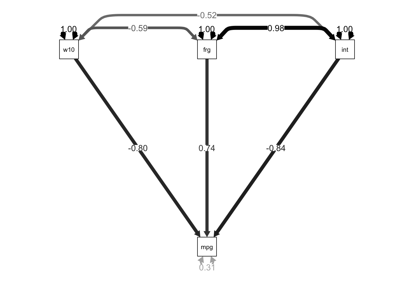
fitted(path.fit)## $cov
## mpg wg1000 foregn int
## mpg 33.020
## wgt1000s -3.580 0.596
## foreign 1.033 -0.209 0.209
## int 1.838 -0.431 0.484 1.1742.7 Nonrecursive models
- these models cannot be fit unless use use special methods like instrumental variables